Black-Box vs White-Box : Differences & similarities

What I find puzzling at times is the ambivalence that process engineers exhibit towards data-driven approaches. On the one hand, use of data is accepted if it’s for regressing First-Principle models (models build on the basic assumptions of the conservation of mass and energy.) On the other hand, if we use the same data to train Black-Box models, we get skeptical faces and great doubt: Will this model be accurate enough? How much can I trust this model’s predictions? I don’t understand whats going on inside that Black-Box!

In this article I would like to share my view on this topic, and how I see both approaches as being two sides of the very same coin.

Most of the time we decide to regress (don’t ever call it train) a first-principle model with measurement data. But what is actually the difference compared to training a black-box model? A first-principle model tries to represent the input/output relationship between some measurements and targets with a set of predefined equations or functions. In essence, what we engineers do in selecting the model based on our understanding of the problem domain is similar to taking a pre-trained black-box model that has certain weights set to zero and suitable kernel functions (sometimes nonlinear) hand-picked by someone else.

Black-Box models

Take a look at the famous feedforward multilayer perceptron model, that still serves as the basis for most neural networks out there. This model, in essence, boils down to a directed, acyclic graph (DAG). When given certain inputs, one can follow the connections defined by the weights and perform the calculation steps prescribed by the activation functions, until one arrives at the output layer.

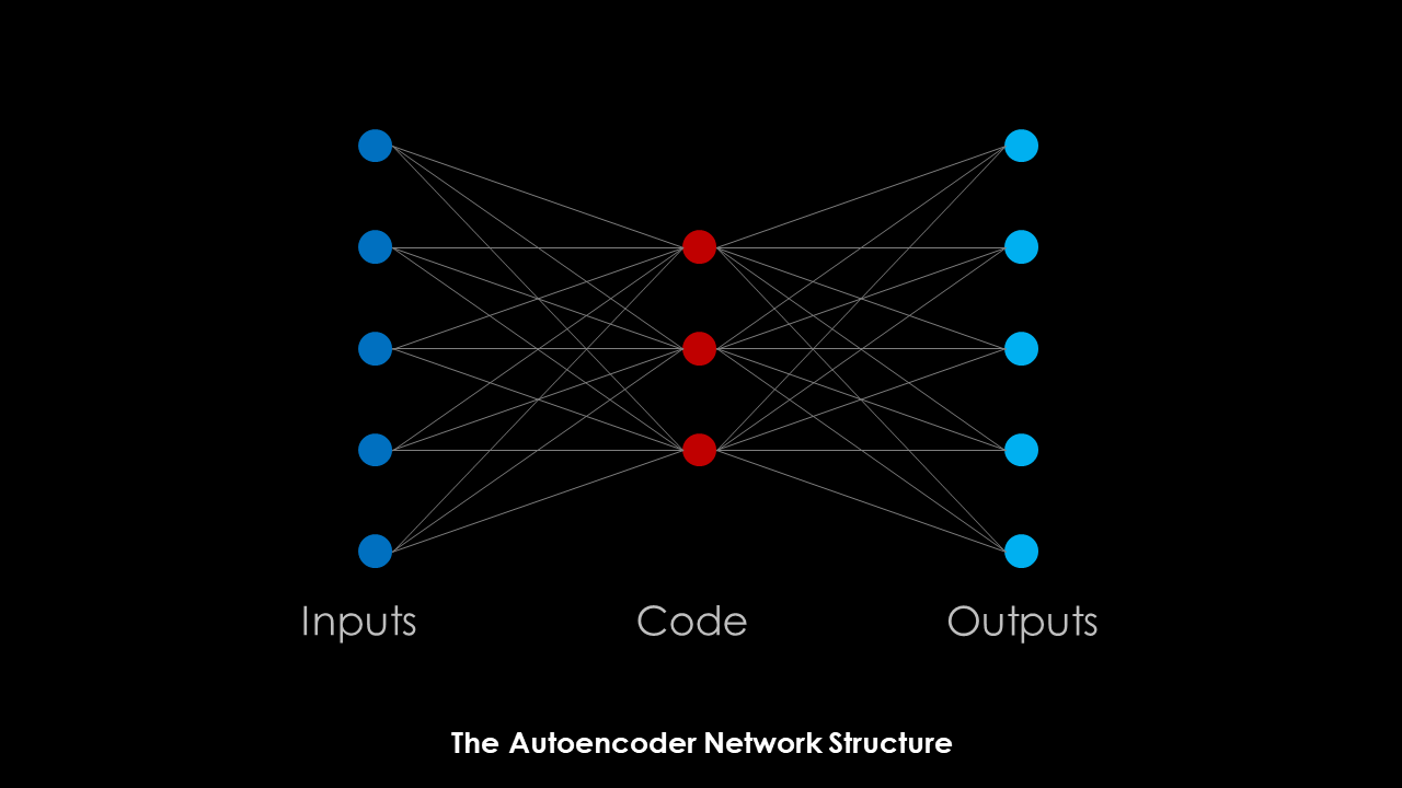
On famous example of a feedforward neural network is the Autoencoder. This network can be summarized as follows:

An autoencoder is a type of artificial neural network used to learn efficient data codings in an unsupervised manner. The aim of an autoencoder is to learn a representation (encoding) for a set of data, typically for dimensionality reduction, by training the network to ignore signal “noise”.

Along with the reduction side, a reconstructing side is learnt, where the autoencoder tries to generate from the reduced encoding a representation as close as possible to its original input, hence its name.

Excerpt from the Wikipedia article

Below you can find a (very simplified) schematic of the architecture of an Autoencoder. The input space is rendered down to a code of reduced dimensionality, from which the outputs can be recreated.

From my point of view, the Autoencoder serves as a perfect example of what first-principle models should do : represent a complex relationship with a set of equations with reduced dimensionality without too much noise. But the Autoencoder does it in a very generalized way without assumptions on the equations describing the relationship or necessary manual steps. In a way, the autoencoder combines the steps of model generation and regression into one coherent framework. Even the hyperparameters like number of layers, number of neurons and types of activation functions can be subject to the training process.

Coming from a background of process design, this nearly sounds like a superstructure that includes all possible programs in its encoding, and the optimizer just has to find the one that represents the problem best.

First-Principle models

In the previous section I tried to explain that Black-Box models try to solve the same problem as First-Principle models, but have the benefit of being much easier to automate because of their simpler structure and less a priori decisions required by the modeler. As a downside, the required numerical effort to regress larger Black-Box Models is much higher, compared to First-Principle models due to the increased number of parameters.

While I mentioned that Neural Networks can be expressed as DAGs, the very same can be said for any expression that we use to write our first-principle model equations. They can be represented as DAGs too, and the same principles can be applied for the evaluation, training or regression.

As an example, examine the valve flow resistance equation. The goal is to calculate the valve coefficient KV from a desired volumentric flow Q and a pressure difference p1-p2. This is a design problem: find equipment sizing parameters from required process conditions. In the picture below I have taken this equation and written it in the form of a DAG. I used the same coloring conventions as for the neural network diagram above, so dark blue nodes represent inputs, red nodes represent calculation nodes and light blue nodes are outputs.

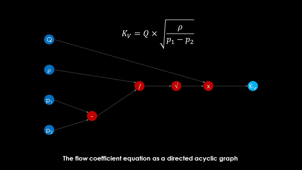
What becomes apparent is that manually constructed graphs are typically much sparser than learned networks. The equation could be described by a neural network with four hidden layers of four nodes each, every node exhibiting one of the activation functions hinted at in the picture: Subtraction, Division, Square-Root, Multiplication. Finding the computation order would then just be an exercise of finding the right weights to connect the neurons in a sensible manner.

By fixing certain functional dependencies a priori using domain knowledge, we reduce the search space so much, that the regression problem becomes tractable. With less parameters to regress, the model is less prone to overfitting, and generally requires less measurements for an acceptable prediction.

As a side node, another way to generate such a DAG without manually fixing the equation structure would be a dynamic programming problem, in which the objective is to construct an expression graph that represents the output values optimally for given inputs. The actual connections and mathematical operations of that graph would be found by an optimization algorithm, taken from a pre-defined set of possible alternatives.

Bringing both worlds together

In the first part of this article I mostly talked about the similarities of both modeling approaches. What are the differences, then?

Well, first of all black box models most often imply some kind of causality. The notion of inputs and outputs are fixed and solving the inverse problem, i.e. calculating the required inputs for a given output requires some sort of iterative method. First-principle models, if formulated in an equation-based form require an iterative solution method from the start on, but are more flexible, as the DAG can be reconstructed for any given set of fixed inputs and calculated outputs. While we don’t get the execution speed of feedforward DAG evaluations most of the time, equation-based first principle models are highly re-usable, as the user can switch the meaning of the variables from input to output easily.

But what happens when we implement a black-box model in mathematical form inside an equation-oriented modeling environment?

In that case, we can switch around the semantics of the variables at will, and rely on the reformulation capability of the modeling environment to perform the matching and sequencing for us. If implemented correctly, we get the regularity of the equation structure of a black-box models (convolutions of nonlinear activation functions and weighted sums of the inputs) and the execution speed of feed forward calculation. Once the equations and variables are matched, the corresponding DAG can be calculated in an efficient way.

Most equation-based modeling languages like GAMS, AMPL, gPROMS, Aspen Custom Modeler, SimCentral or Modelica already perform symbolic analysis on the expression tree level. One implementation of Neural Networks in the language Modelica can be found in this conference article.

Practical Example

I have implemented a very simple example of a feedforward neural network as a unit operation inside my toy-simulator MiniSim. Additionally I created a small example Jupyter Notebook that shows how the structure of the Neural Network can be reorganized to switch input and output semantics, as soon as it is implemented in an open-equation framework.

In this example, it becomes obvious that the entire network can be calculated as a sequence of 6 independent equations, no matter what are the inputs or the outputs. Using Dulmage-Mendelsohn decomposition, the perfect matching is identified and the decomposed system is solved as a serious of assignment statements.

The following code shows how a simple NeuralNet unit is added to a MiniSim flowsheet and bound to other variables (which could, in a realistic example, come from any other stream or unit).

a = expr.Variable("a", 1.0)
b = expr.Variable("b", 1.0)
z = expr.Variable("z", 1.0)

net = NeuralNet("NN1", 2, 1, 1)

net.BindInput(0, a) \
    .BindInput(1, b)\
    .BindOutput(0, z)

solver =  num.DecompositionSolver(logger)
flowsheet = Flowsheet("Test: Neural Net")

flowsheet.AddCustomVariable(z)
flowsheet.AddUnit(net)

status = solver.Solve(flowsheet)
...

When that cell is executed in the Jupyter Notebook, the following output will appear.

Decomposition Result: V=6, E=6, Blocks=6, Singletons=6
Block Statistics:
   # Var # Blocks % Blocks
       1        6 100,00 %
Problem NLAES was successfully solved (0,04 seconds)

Solve equation EQ000005 >> 0 := U[1] - b = 0 for variable U[1]
Solve equation EQ000004 >> 0 := U[0] - a = 0 for variable U[0]
Solve equation EQ000001 >> 0 := u[0,0] - ((1 * U[0] + 1 * U[1]) + 0) = 0 for variable u[0,0]
Solve equation EQ000002 >> 0 := y[0,0] - 1 / 1 + exp(-(u[0,0])) = 0 for variable y[0,0]
Solve equation EQ000003 >> 0 := Y[0] - (1 * y[0,0]) = 0 for variable Y[0]
Solve equation EQ000006 >> 0 := Y[0] - z = 0 for variable z

a=1.0
b=1.0
z=0.8807970779778823

In the output we see that the system was decomposed into 6 sub problems, each consisting of one variable and one equation: a perfect matching was found. The equations can be solved one after another, and then the result is used for the calculation of the next variable.

The neural net thus responds with an output z~=0.881 for the inputs a=1 and b=1.

You can see a symbolic representation of my experiment in the picture below. If you fix (or free) a variable (or parameter) in an equation-oriented framework, you just “switch” the direction of the information flow. Whereas before we calculated z from a and b, we can now calculate what the value of a must be, when b and z are given.

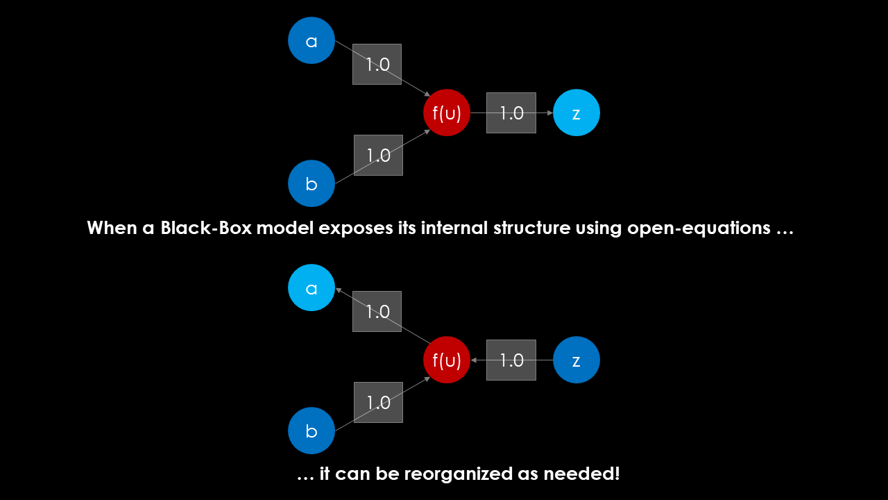
In the Jupyter Notebook you can see how a decomposition solver reorganizes the equations to solve a series of 6 1x1 systems, even though it has to solve an inverse problem now.

Summary

I believe that the modeling capabilities of process simulators can be expanded greatly, if they would support internal implementations of typical black-box models, essentially opening up the box and exposing the equation structure within.

Only when equation-oriented solvers can efficiently exploit the structure of Black-Box models, we can truly integrate those models (which might even be trained outside of the simulator using a machine-learning toolchain of your choice) into existing flowsheet simulations. When that happens, we have a new, flexible, robust and powerful building block in our modeling repertoire.