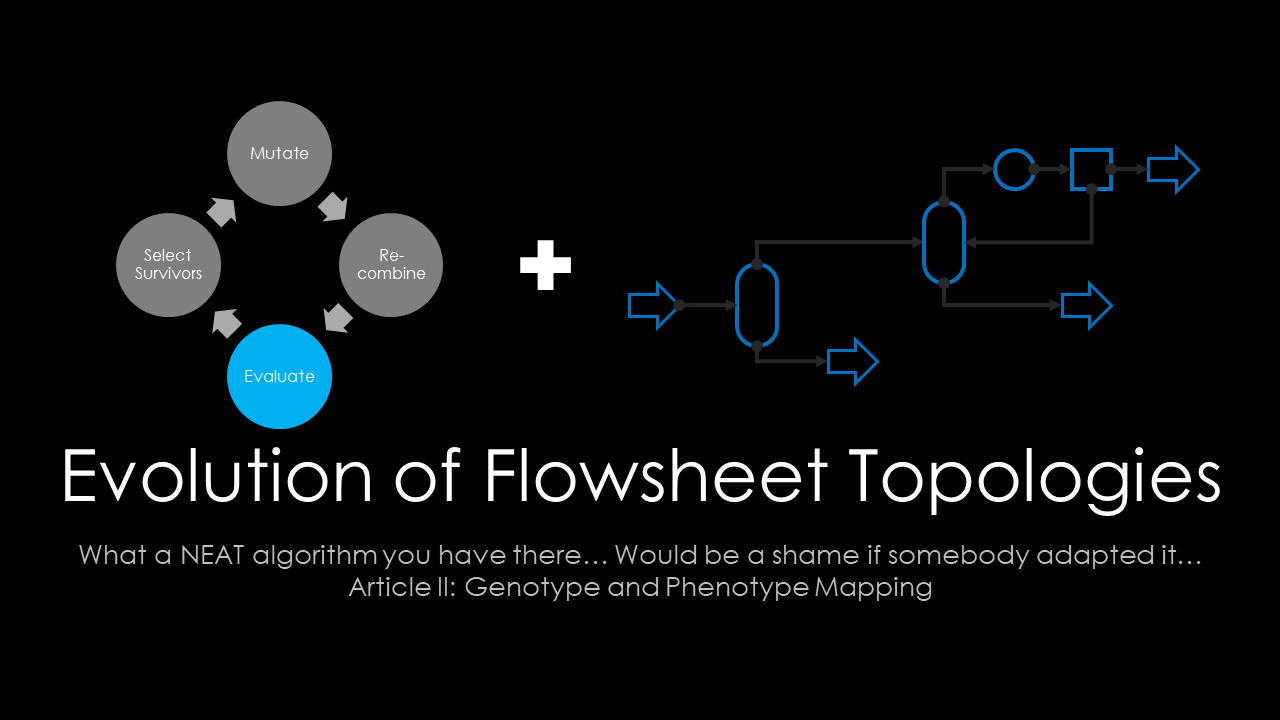
Evolution of flowsheet topologies - Part 2: Genotype and Phenotype Mapping

The most important design decisions regarding an evolutionary algorithm come up when the encoding method is defined. Where historical approaches commonly used bit-strings for encoding decisions (or even floating-point numbers), in the last few years more complex data models have emerged. The genome encoding heavily influences the effort needed for the implementation of the evolutionary operators like mutation, and cross-over.

In my past endeavors on this topic (available here or here) I used evolutionary strategies that encoded the search space as fixed-length genomes of binary, integer or continuous variables. With a fixed-length genome mutation and cross-over operators can be implemented easily. For mutation, I iterated over the genes and with a certain chance, modified the value according to some random distribution function. For cross-over I used a simple one-point crossover that chose a random gene and then exchanged the gene sequences left and right of the cross-over point for the parent genotypes.

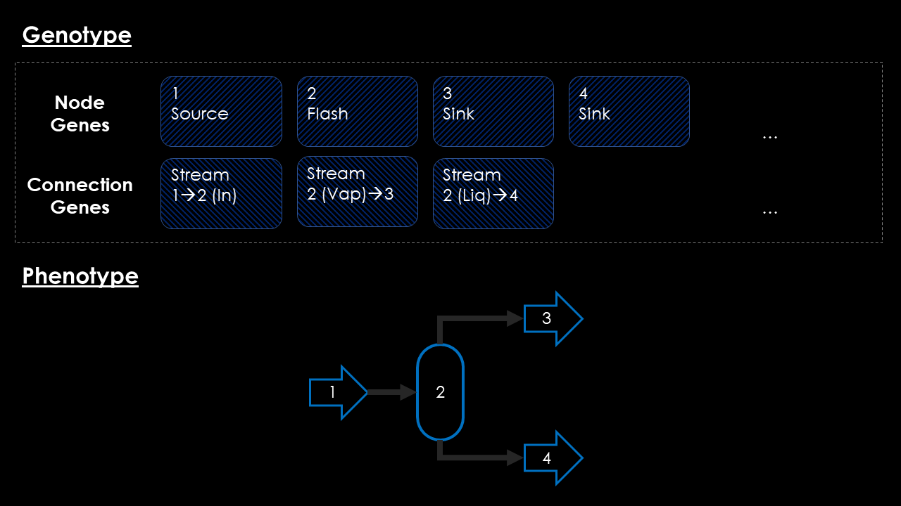
The Neuro-Evolution of Augmented Topologies Algorithm uses a different approach though. Inspired by this algorithm in this project I will use a random-length genome consisting of two different chromosomes. One chromosome will hold the information about the unit operations used in the design candidate, while another chromosome will store the information about the connectivity between those unit operations. A conceptual view of this genome and a resulting phenotype mapping is shown in the image below.

Neural and Process Networks

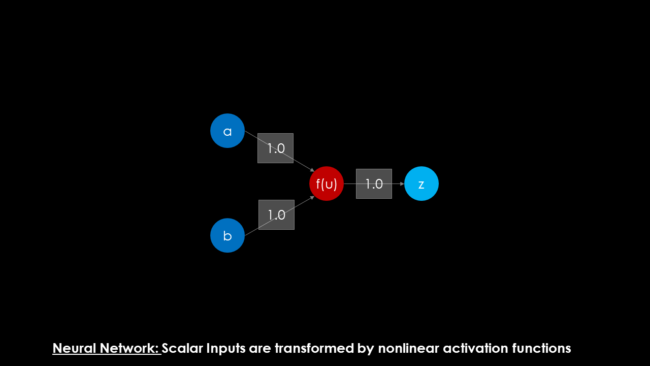
Before the details of this representation are revealed, let me indulge a bit in my reasoning of why I think the NEAT algorithm is so fitting for process synthesis. In the image below, the structure of a standard neuron is given. Multiple scalar valued inputs are fed into a neuron, an input signal is calculated via summation of the signal (and an optional bias is applied) before the input signal is transformed by an (often nonlinear) activation function. The output signal can either be used as an output for the algorithm, or fed to another layer in a network to create deeper convolutions of nonlinear functions.

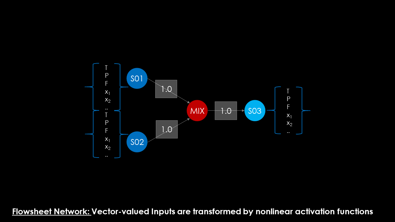
Compare this to a typical process flowsheet. Here, vector-valued inputs (the state variables of the streams) are fed into the unit operation model, in which they are recombined to form the input signal. This operation heavily depends on the actual unit operation: in a mixer, both input signals are summed up, but in a heat exchanger the input signals are only connected by the heat balance. After a series of internal calculation one or more vector-valued outputs are available, to be either propagated to further downstream units or removed from the flowsheet via sinks.

From a conceptual point of view I see a lot of similarities between Neurons and Unit Operation Models. They differ in input structure, the input and the activation function, but share a lot in topological information. Both are directed computational graphs (sometimes with cycles as recurrence is a theme both in Neural Networks and Process Flowsheets) that can be analyzed and solved with similar algorithms.

The major difference lies in the complexity of function evaluation: whereas functions in Neural Networks are nearly always explicit elementary functions, Unit Operation nearly always require an iterative solve procedure before the corresponding outputs can be determined for a given set of inputs. This difference will lead to a drastic increase in calculation time and will furthermore decrease stability of the algorithm, as the iterative procedures may sometimes fail.

The Genotype

At this point we are ready to start our modeling endeavor. To test out the idea of a generic process model that is later translated into a “real” flowsheet, we start with a very simple Python dictionary. I will not deal with any mutation or cross-over but instead fill a data structure manually for testing.

The genotype consists of:

• A counter for the generation
• An ID to identify the individual within the generation
• A list of Unit Genes
• A list of Stream Genes

The UnitGene consists of a class identifier that is used to create UnitOperation instances later, as well as the parameters needed to make the model specification square. We will rely only on the evolutionary search to optimize our process and thus have to make sure that the flowsheet is fully specified. In this example, the thermodynamics system consists of three components, Benzene, Toluene and p-Xylene, which are relabled as component A, B and C respectively. This way, I can easily change the system to any other ternary system and do not need to change the models.

Each unit will have a field called IsMandatory, to tell the mutation operator that such a unit must exist in a flowsheet and cannot be removed. This is neccessary to guarantee that we will always have a feed, an idea that is taken from the work of Thibaut Neveux.

The MaterialStream genome-model is very simple and consists only of a name for the stream, the source unit and port, and the sink unit and port. Splitters and mixers will be modeled explicitly with Unit Operation nodes and not with different weightes streams.

For the start I will model a small flowsheet consisting of two flashes and a condenser to test out the idea. The process task is defined by the composition of the mandatory feed stream: a mixture 30/30/40 mol-% Benzene, Toluene, Xylene needs to separated.

genotype={
    "Generation":1,
    "ID":1,
    "UnitGenes":[
        {
            "ID":"U1",
            "Class":"Feed",
            "IsMandatory":True,
            "Parameters":[ 
                {"Name":"n","Value":100,"UoM": kmolh},
                {"Name":"T","Value":298,"UoM": SI.K},
                {"Name":"P","Value":370,"UoM": METRIC.mbar},
                {"Name":"x[A]","Value":0.3,"UoM": SI.none},
                {"Name":"x[B]","Value":0.3,"UoM": SI.none},
                {"Name":"x[C]","Value":0.4,"UoM": SI.none},
            ]
        },
         {
            "ID":"U2",
            "Class":"Flash",
            "IsMandatory":False,
            "Parameters":[         
                {"Name":"VF","Value":0.5,"Min":0.2,"Max":0.8,"UoM": SI.none},
                {"Name":"P","Value":370,"UoM": METRIC.mbar},
             ]                       
        },
         {
            "ID":"U3",
            "Class":"Product",
            "IsMandatory":False,
            "Parameters":[]                       
        }
        ,
         {
            "ID":"U4",
            "Class":"Product",
            "IsMandatory":False,
            "Parameters":[]                       
        },
         {
            "ID":"U5",
            "Class":"Flash",
            "IsMandatory":False,
            "Parameters":[
                {"Name":"VF","Value":0.5,"Min":0.2,"Max":0.8,"UoM": SI.none},
                {"Name":"P","Value":370,"UoM": METRIC.mbar},
             ]                       
        },
         {
            "ID":"U6",
            "Class":"Heater",
            "IsMandatory":False,
            "Parameters":[
                {"Name":"VF","Value":0,"UoM": SI.none},
                {"Name":"P","Value":370,"UoM": METRIC.mbar},
             ]                       
        },
        {
            "ID":"U7",
            "Class":"Product",
            "IsMandatory":False,
            "Parameters":[]                       
        },
    ],
    "StreamGenes":[
        {"ID":"S1", "From":("U1","Out"), "To":("U2","In")},
        {"ID":"S2", "From":("U2","Vap"), "To":("U6","In")},
        {"ID":"S3", "From":("U2","Liq"), "To":("U5","In")},
        {"ID":"S4", "From":("U5","Vap"), "To":("U3","In")},
        {"ID":"S5", "From":("U5","Liq"), "To":("U4","In")},
        {"ID":"S6", "From":("U6","Out"), "To":("U7","In")},
    ]
}

A working example

I have created a small Jupyter Notebook that shows how a genotype is mapped to a phenotype, which in this case is a Flowsheet object from the MiniSim flowsheet simulator.

The phenotype handling consists of three main algorithms:

• Genotype->Phenotype Mapping: A simple factory method that projects a genotype object (Dictionary) onto a Flowsheet object.

• Phenotype->Objective Mapping: A method that projects a Flowsheet object onto a single scalar value, that can either be an economic objective or (as currently implemented) a surrogate function that will drive the optimization towards the desired direction. The objective function will be featured in a later article in more depth, as it is very important for the evolutionary search.

• Phenotype-Process Flow Diagram Mapping: Two functions that assign positions on a canvas to each Unit Operation and render the flowsheet onto a two-dimensional image. I will need a quick way to generate a pictorial view of the phenotype to debug the mutation and cross-over operators later in the project. Just looking at nodes and vertices will not be enough to see if the results are reasonable from a process engineering point of view.

In the example Notebook, all three algorithms are applied to the genome shown above. The resulting, automatically rendered flowsheet is shown in the image below.

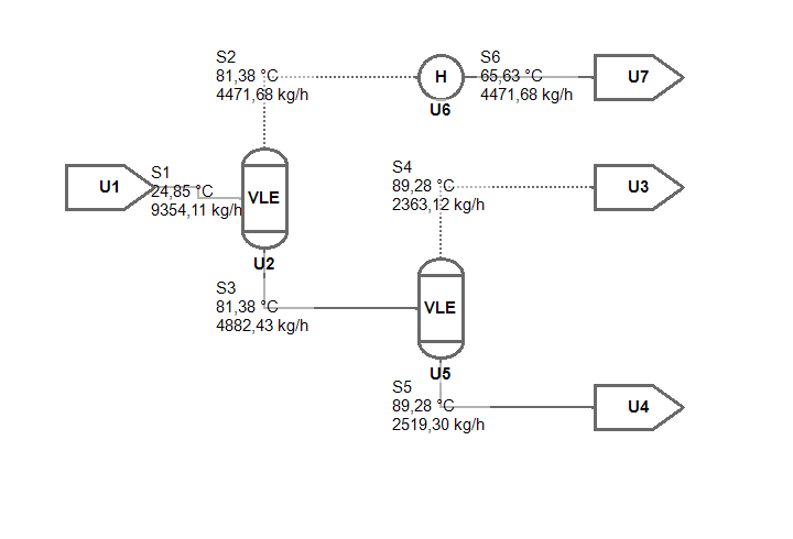
Summary and open questions

The flowsheet shown is actually fully solved already, but this of course relies on a trick. I created the genome manually and could choose the sequence of the Unit Operations. Of course I added the flashes and the heater in such a way, that a straight-forward calculation is possible and the Newton-type solver converges quickly after a trivial initialization.

The next part article will tackle one of the most intricate problems of this whole series: is it possible to find an algorithm that will bootstrap the automatically created flowsheet models so that acceptable convergence rates are achieved in the objective function evaluation phase.

Luckily a lot of research went into the topic of flowsheet tearing and sequencing and the current state of my research looks already promising, except for one thing…

You may have noted that I only used flashes and heaters in the example. While it is of course possible to solve distillation columns with MiniSim, I haven’t found a convincing way of including them in the genome. Currently I am pondering two options, but cannot decide which one I should pursue further.

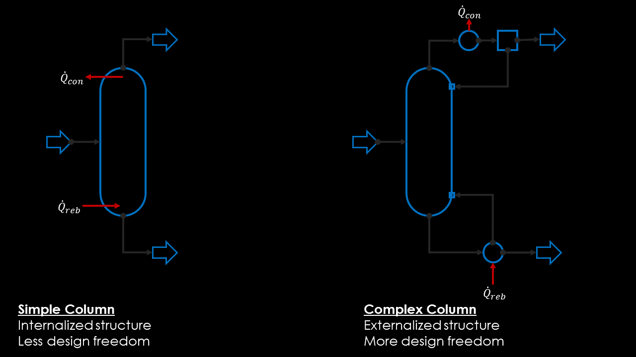
• Option A: If I model them only as simple distillation with a single feed and two product streams, startup will be easier, but I lose a lot of potential solutions (heat-integrated columns, dividing wall setups, absorbers or stripping columns).
• Option B:If I model them as adiabatic sections, I need to add additional sources for the boilup and liquid reflux. How to initialize those streams still is an open question to me.

So until next time, stay tuned and contact me if you have any questions or remarks. I would be happy to discuss the topic adressed in this post with anyone interested.