Evolution of flowsheet topologies - Part 3: Automatic flowsheet initialization

In my last article I mentioned an unsolved challenge that needs to be discussed before I can start to actually implement the evolutionary algorithm itself:

It needs to be shown that an algorithm can be found that, using a numerical solver, evaluates the arbitrary process designs that will be generated by the evolutionary algorithm by mutation and cross-over.

Anyone with a background in process simulation can attest to the difficulty of getting process flowsheets to converge, especially if they exhibit distillation columns and recycles. This challenge is even harder with equation-oriented simulators, which have to rely on a general-purpose algorithms to solve the mass- and energy balance and cannot use tailored algorithms for each unit, unlike sequential-modular simulators.

A good comparison of these two approaches can be found on the homepage of PSE, the well known vendor of the gPROMS modelling & simulation software. PSE has developed a lot of initialization routines for the equation-oriented simulator gPROMS, but they are generally considered secrets and are not discussed publicly.

If one goes back in time into the 1970ies and 1980ies, a lot of literature shows up that deals with the problem of solving simulation flowsheets. Limited numerical capabilities of the time required “intelligent” algorithms that exploited the structure of the problem to speed up the solution time.

Although many of these ideas were originally intended to be used within a sequential-modular simulators, one can easily adapt them to an equation-oriented simulator if it is possible to quickly generate sub-equation-sets consisting only of a single unit.

First steps and trivial initialization

The simulator available to me, my toy simulator MiniSim, only supports an equation-oriented (EO) modeling approach and solves the resulting nonlinear algebraic equation systems using a (heuristically modified) Newton-Raphson solver (you can find the code here).

It has all the problems associated with an EO solver such as difficult startup from arbitrary initial conditions. Luckily I have full control over the source code of MiniSim as it is an Open-Source project and can add new features easily. One extension was to add problem-specific Initialize() methods to each unit operation class. Inside these methods I wrote specific algorithms to pre-calculate the state variables using simple Flash routines and hard-coded mass-balances. As these algorithms have to be hand-written, I can only support a limited set of specifications. But anyway, I will solve the “real” flowsheet using an equation-oriented solver later, so a good initial guess is fine.

Furthermore, the user of MiniSim is able to create light-weight instances of Equation Systems very easily. Based on that feature, I added a Solve() method to each unit operation class, that will create a minimal equation system consisting just of the equations and variables of the unit operation as well as those of the outgoing streams. This small equation system is then solved using a Dulmage-Mendelsohn Decomposition-based solver that automatically determines a matching between variables and equations and solves them one at a time.

If the Initialize() and Solve() methods are called in succession, the model has quite reasonable initial values, that in many cases result in acceptable convergence rates for the overall problem.

Now that we are able to solve units one-by-one, or “sequential-modular”, we only need one building block for a robust calculation: the right sequence.

Sequencing and tearing

A LOT has already been written about the subject of flowsheet tearing. If you want to know more about this topic, refer to the works of Varma, Lau and Ulrichson, Motard and Westerberg or Gundersen.

When talking about process flowsheets, one cannot dismiss graph theory. Any process flowsheet can be represented by a directed graph consisting of flowsheet units (nodes) and streams (vertices). The challenge is to find a topological sorting of the graph. While this is easy to determine for a directed acyclic graph, process flowsheet very often have recycle streams that form closed cycles. These cycles have to be torn, and you need to decide which stream to tear. Tear streams (or sets of tear streams) are not unique, which might explain the multitude of tearing algorithms, as each algorithm has different criteria for selecting the optimal tear set.

A simple example

I have created a Jupyter Notebook with an example to test out my ideas for a simple tearing algorithm. It uses the flowsheet of a pressure-swing distillation for separating methanol and acetone. This process features two distillation columns and a recycle flow from the second column to the first and was adapted from a ChemSep simulation, which in turn is based on a paper by Luyben.

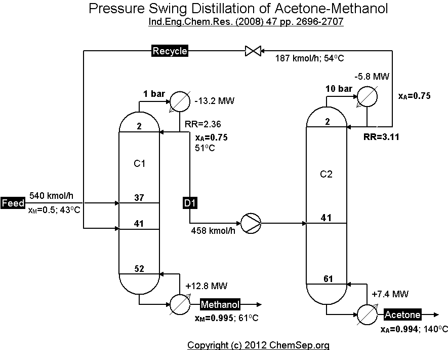
Remark: Due to the way rendered flowsheets are converted to Jupyter images, they are saved as raw bitmaps with Base64 encoding. This results in very large Jupyter Notebooks. You might have to clone the entire repository to view the Notebooks, as the Notebook Viewer of Github sometimes refuses to render to large files. I need a way to compress the image before they are stored as Base64 strings in the Notebook file but so far haven’t been successful.

I decided to go with my own tearing algorithm because the existing ones are rather convoluted and are geared to find sequences that can be solved with the minimal amount of evaluations in a sequential-modular simulator. As I only need good initial guesses, I can accept an algorithm that would take long to converge, because I abort it long before it would converge naturally.

I will not go into the details of the implementation, which you can see in the Jupyter Notebook. In short, the algorithm performs the following steps:

• Using Tarjan’s algorithm for strongly connected components the strongly connected components (SCC) are detected and a coarse sequence of units and sub-flowsheets that can be solved sequentially is generated.
• The coarse sequence is iterated over:
  • If an element is a single unit operation, it is added to the final calculation sequnece.
  • If an element is a SCC the strongly connected component is torn by adding only those unit operations to the calculation sequence that have the most direct predecessors already in the calculation sequence.
    With this heuristic a unit is initialized only when most of its upstream units are already solved. When a unit is added to the sequence, other units now have their requirements fulfilled and can be added to the sequence themselves.
• Step 2 is repeated until all strongly connected components are empty and all unit operations of a flowsheet are part of the final calculation sequence.

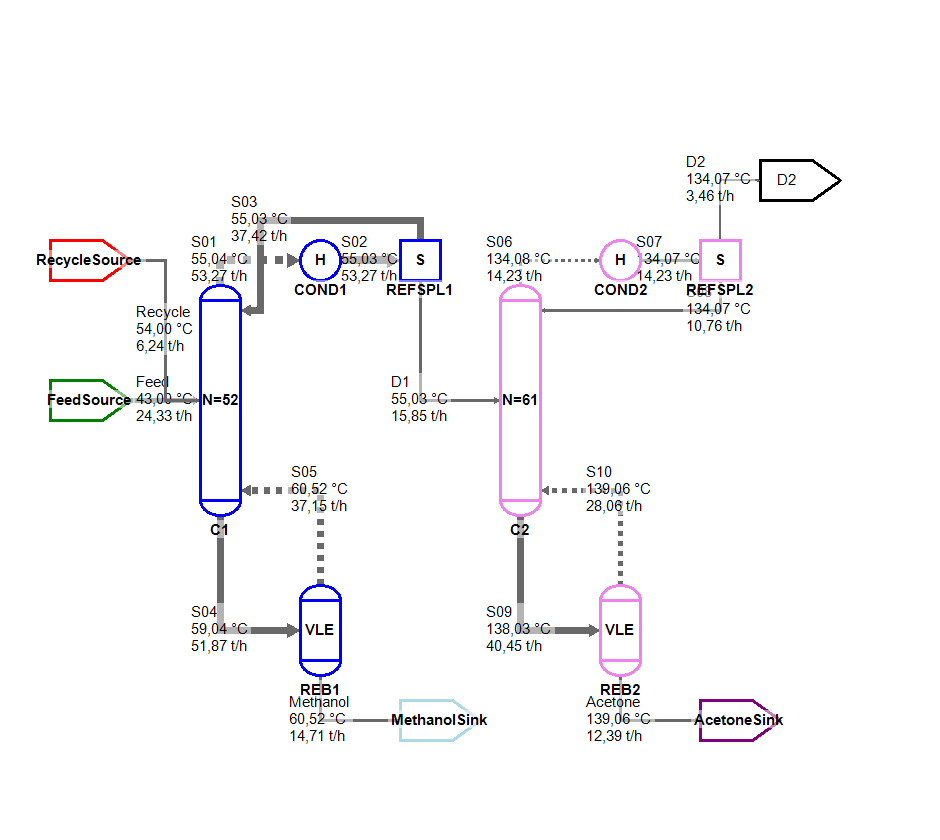
In the image below you can see the results of the strongly connected component algorithm for this case study when the recycle stream is manually torn: Each source and sink can be solved individually (indicated by the border color), whereas each distillation column with periphery (condenser, reflux splitter and reboiler) would have to be solved as one SCC.

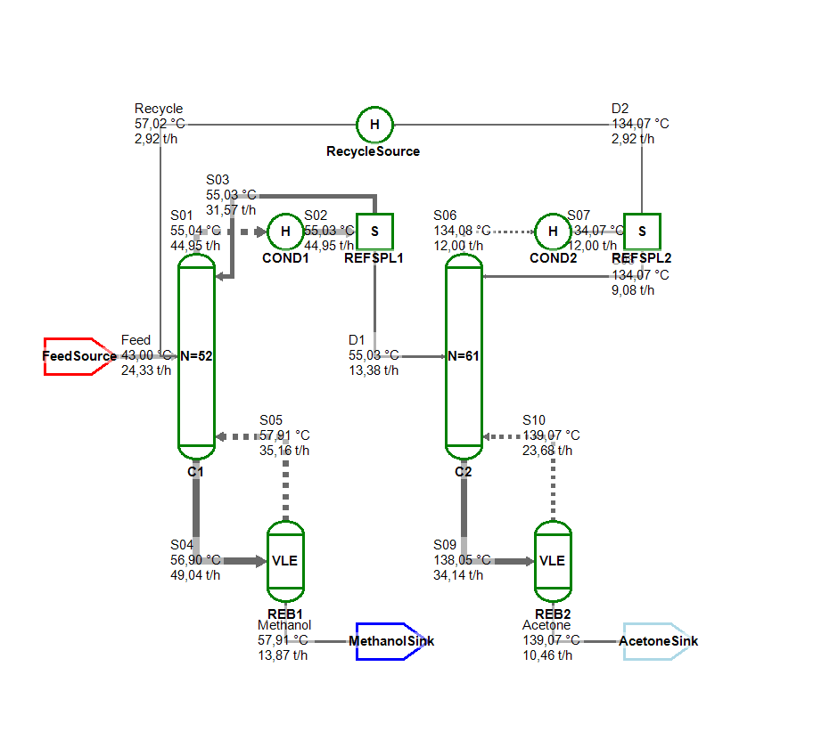
If the recycle stream is connected, both columns are part of the same strongly connected component (indicated by the green borders). But even in this case, which features 5 cycles, the simple heuristic works quite well and the flowsheet can be solved quickly. It might be required to perform multiple (3-5) initialization passes to be sure that every unit was calculated with reasonable inputs at least once.

From fixed flowsheets to genomes

My end goal is to create flowsheet topologies from simpler data structures that encode the flowsheet with only a few numbers. I talked about the Genome in an earlier article, and this time I added the ability to encode Distillation columns.

In the last article I still debated myself if I should encode distillation columns as adiabatic sections or simple columns (with reboiler and condenser).

I decided to go with alternative B. I just could not find a way to find reasonable values for the vapor and liquid reflux inlets if I could not assume the existence of a reboiler or condenser. What composition should the vapor have? What should the reflux look like? Pure solvent? Should it resemble to feed? I just don’t know yet. While I will lose some solutions from the design space, I can at least calculate some designs already now, and maybe I can find a way to add absorbers or stripping columns to the genome later in my article series.

You can find the extended mapping algorithm in another Jupyter Notebook. Here I hand-crafted a simple genome describing two distillation columns in sequence. In the image below you can see that the sequencing algorithms is applied to the resulting phenotype and the algorithm can actually solve this flowsheet very easily.

A first step into the random

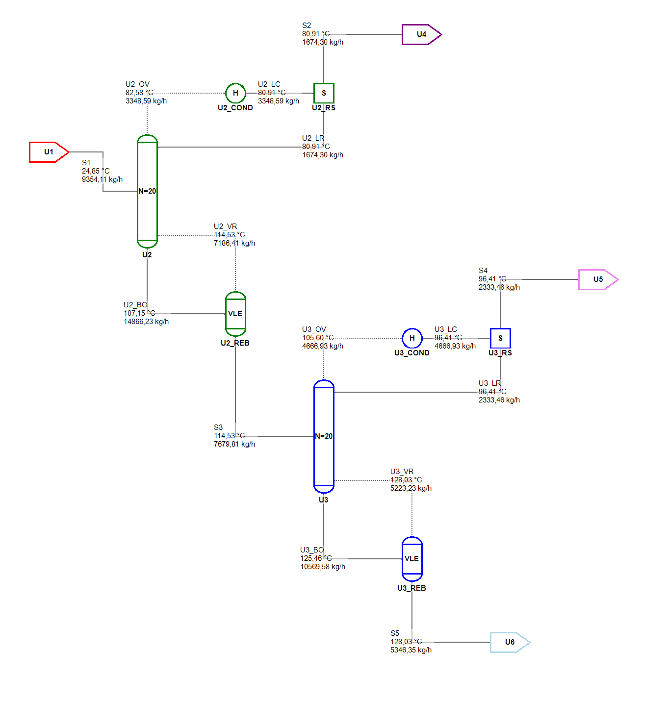
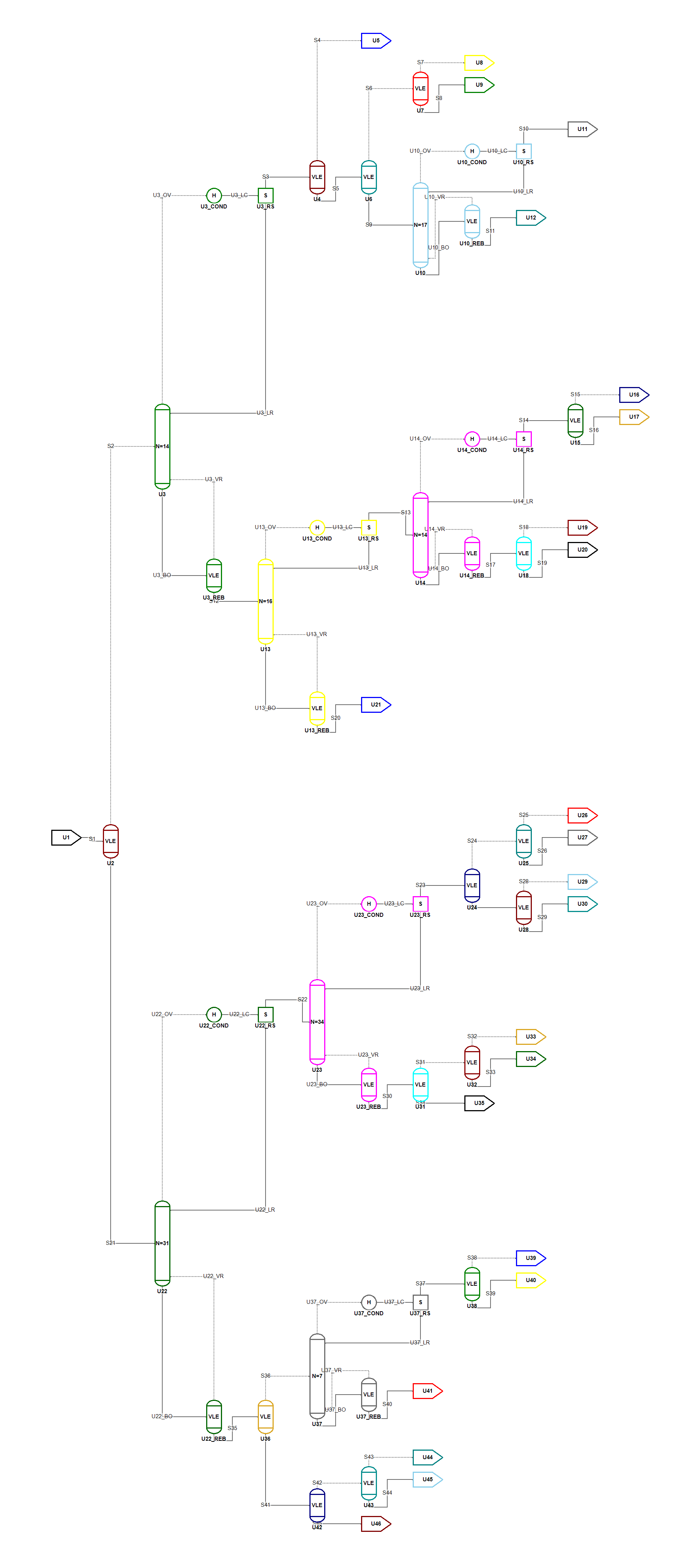
Now that I was confident that I could represent distillation columns in the genome and solve the resulting flowsheet models I build yet another small Jupyter Notebook that generates random flowsheets consisting of flashes and distillation columns up to a pre-defined depth.

One such randomly generated flowsheet can be seen in the picture below. Once again the Tarjan’s algorithm performs its magic and a reasonable sequence can be identified and the flowsheet can be solved quite easily even with a toy simulator like MiniSim.

Conclusion

In this article I have solved and discussed some of the open questions of this article series:

• A simple heuristic algorithm that sequences an arbitrary flowsheet and performs a generalized start-up routine was described and implemented.
• A way to represent distillation columns in the genome was defined and the Genotype-to-Phenotype mapping algorithm was modified to create flowsheet instances containing distillation columns.
• A randomized algorithm was described and implemented that creates feasible (albeit non-sense) flowsheet designs from scratch.

The next articles will cover the following topics:

• How to create an actual mutation function that creates new flowsheet designs from existing ones?
• How to find suitable objective functions for comparing different designs?
• How to transfer the ideas of cross-over and speciation from the NEAT algorithm to the problem domain of flowsheet topologies?

So until next time, stay tuned and contact me if you have any questions, remarks or ideas. I would be happy to discuss the topic adressed in this post with anyone interested.

Written on January 28th, 2020 by Jochen Steimel